Simulation and modeling 2073
Group A
Long Answer Questions:
Attempt
any two questions.
(2x10=20)
1. Define and describe Markov chain in detail with the help of suitable examples. Also describe at least three areas of application of Markov chain.
If the future states of a process are independent of the past and depend only on the present , the process is called a Markov process. A discrete state Markov process is called a Markov chain. A Markov Chain is a random process with the property that the next state depends only on the current state.
Markov chains are used to analyze trends and predict the future. (Weather, stock market, genetics, product success, etc.
Formally,
A Markov chain is a sequence of random variables X1, X2, X3, ... with the Markov property, namely that, given the present state, the future and past states are independent.

The conditional probability above gives us the probability that a process in state in at time n moves to in+1 at time n + 1. We call this the transition probability for the Markov chain. If the transition probability does not depend on the time n, we have a stationary Markov chain, with transition probabilities

Now we can write down the whole Markov chain as a matrix P:

Example:
Weather Problem:
- raining today ⇒ 40 % rain tomorrow
⇒ 60 % no rain tomorrow
- not raining today ⇒ 20 % rain tomorrow
⇒ 80 % no rain tomorrow
What will be probability if todays is not raining then not rain the day after tomorrow?
Markov chain diagram:

Transition matrix:


Thus, the probability of not rainy the day after tomorrow is 0.76.
Applications of Markov Chain
1. Physics: Markovian systems appear extensively in thermodynamics and statistical mechanics, whenever probabilities are used to represent unknown or unmodelled details of the system, if it can be assumed that the dynamics are time-invariant, and that no relevant history need be considered which is not already included in the state description.
2. Internet applications: The Page Rank of a webpage as used by Google is defined by a Markov chain. It is the probability to be at page i in the stationary distribution on the following Markov chain on all (known) web pages
3. Statistics: Markov chain methods have also become very important for generating sequences of random numbers to accurately reflect very complicated desired probability distributions, via a process called Markov chain Monte Carlo (MCMC) And many more.
2. Define and develop a Poker test for four-digit random numbers. A sequence of 10,000 random numbers, each of four digits has been generated. The analysis of the numbers reveals that in 5120 numbers all four digits are different, 4230 contain exactly one pair of like digits, 560 contain two pairs, 75 have three digits of a kind and 15 contain all like digits. Use Poker test to determine whether these numbers are independent. (Critical value of chi-square test for α=0.05 and N=4 is 9.49)
The Poker Test is the test for independence based on the frequency with which certain digits are repeated with in a series of numbers. This test not only tests for the randomness of the sequence of numbers, but also the digits comprising of each of the numbers. The expected value of each of the combination of digits in a number is compared with the observed value by means of the chi-square test for independence. The acceptance is done if the observed value of chi-square sums for all the possible combinations of digits is less than the acceptable value for the given degree of freedom at the specified confidence interval.
Poker test for four digit numbers
In four digit number, there are five different possibilities
- All individual digits can be different
- There can be one pair of like digit
- There can be two pair of like digits
- There can be three digits of a kind
- There can be four digits of a kind
The probabilities associated with each of the possibilities is given by
P (four different digits) = 4C4 * (10/10) * (9/10) * (8/10) * (7/10) = 0.504
P (one pair) = 4C2 * (10/10) * (1/10) * (9/10) * (8/10) = 0.432
P (two pair) = (4C2/2)*(10/10) * (1/10) * (9/10) * (1/10) = 0.027
P (three digits of a kind) = 4C3 * (10/10) * (1/10) * (1/10) * (9/10) = 0.036
P (four digits of a kind) = 4C4 * (10/10) * (1/10) * (1/10) * (1/10) = 0.001
Now the calculation table for the Chi-square statistics is:
| Combination(i) | Observed Frequency(Oi) | Expected Frequency(Ei) | (Oi-Ei) | (Oi-Ei)2/Ei |
| Four different digits | 5120 | 0.504*10000 = 5040 | 80 | 1.269 |
| One pair | 4230 | 0.432*10000 = 4320 | -90 | 1.875 |
| Two pair | 560 | 0.027*10000 = 270 | 290 | 311.481 |
| Three digits of a kind | 75 | 0.036*10000 = 360 | 285 | 225.625 |
| Four digits of a kind | 15 | 0.001*10000 = 10 | 5 | 2.5 |
| 10000 | 10000 | Σ(Oi-Ei)2/Ei = 542.75 |
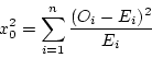 = 542.75
and Given  α, N = 0.05, 4= 9.49
Here the calculated value of chi-square is 542.75 which is greater than the given tabulated value of chi- square so we reject the null hypothesis of independence between given numbers.
3. Define congestion. Describe different types of components, characteristics and queueing disciplines of a queueing system.
A congestion system is system in which there is a demand for resources for a system, and when the resources become unavailable, those requesting the resources wait for them to become available. The level of congestion in such systems is usually measured by the waiting line, or queue, of resource requests (waiting line or queuing models).
Characteristics/Elements of Queueing System
The key elements of queuing systems are customer and server. Customer refers to anything that arrives at a facility and requires service. E.g. people, machines, trucks, emails. Servers refers to any resource that provides the requested service. E.g. receptionist, tellor, CPU, washing machine etc.
1. Calling Population
The population of potential customers those require service from system is called calling population. It may be finite or infinite. System having large calling population is usually considered as infinite. For e.g. customers at banks, restaurant. And System having less and countable population is usually considered as finite. For e.g. a certain number of machines to be repaired by a service man.
In finite population model, arrival rate depends on the number of customers being served and waiting. But in infinite population model, arrival rate is not affected by the number of customer being served and waiting.
2. Arrival Process
The arrival process for infinite-population models is usually characterized in terms of interarrival times of successive customers. Arrivals may occur at scheduled times or at random times. When at random times, the inter arrival times are usually characterized by a probability distribution and most important model for random arrival is the poisson process. In schedule arrival interarrival time of customers are constant.
3. Service Process
Service process can be measured by the number of customers served per some unit of time or the time taken to complete the service. Once entities have entered to the system they must be served. The service can be provided in single or batch. if it is batch, as in the case of arrival the batch size can be fixed or random. Service time may be of constant duration or of random duration.
Markov Service process: A Markov service process is a special service process in which entities are processed one at a time in FCFS order and service times are independent and exponential. Aswith the case of Markov arrivals, a Markov service process is memoryless, which means that the expected time until an entity is finished remains constant regardless of how long it has been in service.
4. Queueing Discipline and Queueing Behaviour
Queue discipline refers to the rule that a server uses to choose the next customer from the queue when the server completes the service of the current customer. Common queue disciplines include first-in-first-out (FIFO); last-in-first-out (LIFO); service in random order (SIRO); shortest processing time first (SPT); and service according to priority (PR).
- First in first out :This principle states that customers are served one at a time and that the customer that has been waiting the longest is served first.
- Last in first out : This principle also serves customers one at a time, however the customer with the shortest waiting time will be served first.
- Service in random order: A customer is picked up randomly from the waiting queue for service.
- Shortest job first: The next job to be served is the one with the smallest size (shortest service time).
- Priority: Customers with high priority are served first.
Queue behavior refers to the actions of customers while in a queue waiting for service to begin. Different queue behaviours are:
- Balk/Balking: It means leaving the queue when the customer see the line is too long.
- Renege/Reneging: Leave after being in the line when they see that the line is moving too slowly.
- Jockey/Jockeying: Move from one to a shortest line.
5. Number of Servers:
Servers represent the entity that provides service to the customer. A system may consist of single server or multiple servers.
- A system with multiple servers is able to provide parallel services to the customers.
Group B
Short answer Questions:
Attempt
any eight questions. (5x8=40)
4. Define model. Describe different types of simulation models in brief.
Model is a computerized program that defines the mechanics of the considered system. It must have state which may change on each time step. Model represents the system for the purpose of studying the system.
A simulation model can be classified as being static or dynamic, deterministic or stochastic, and discrete or continuous.
- A static simulation model, sometimes called a Monte Carlo simulation, represent a system at a particular point in time. For example, the profit of a company, which is affected by 3 variables drawn from different statistics distributions.
- A dynamic simulation model represents a system as it changes over time. For example, the simulation of a bank from 9 am to 4 pm.
- Deterministic model contains no random variables. They have a known set of inputs which will result in a unique set of outputs. E.g. Arrival of patients to the Dentist at the scheduled appointment time.
- Stochastic model has one or more random variable as inputs. Random inputs leads to random outputs. E.g. Simulation of a bank involves random inter-arrival and service times.
- Discrete model is one in which the state variables changes only at a discrete set of time. For example: banking system in which no of customers (state variable) changes only when a customer arrives or service provided to customer i.e. customer depart form system.
- Continuous model is one in which the state variables change continuously over time. For example, during winter seasons level of which water decreases gradually and during rainy season level of water increase gradually. The change in water level is continuous.
5. Describe the importance of differential/Partial differential equations in simulation.
The equation that consists of the higher order derivatives of the dependent variable is known as differential equations.
- The differential equation is said to be linear if any of the dependent variables and its derivatives have power of one and are multiplied by the constant.
E.g. M x’’ + D x’ + K x = K F(t)
where, M, D and K are constants; F(t) is the input to the system depending upon the independent variable t; x’’ and x’ are second and first order derivatives of dependent variable x.
- The differential equation is said to be non-linear if the dependent variable or any of its derivatives are raised to a power or are combined in other way like multiplication.
The differential equation is said to be partial if more than one independent variables occur in a differential equation.
-E.g. Equation of flow of heat in three dimensional body. It consists of four independent variables ( three dimensions and time ) and one dependent variable ( temperature ).
Necessity of differential equations:
1. Most physical and chemical process occurring in the nature involves rate of change, which requires differential equations to provide mathematical model.
2. It can be used to understand general effects of growth trends as differential equations can represent a growth rate.
6. What do you understand by interactive system? Explain
Interactive systems are computer systems characterized by significant amounts of interaction between humans and the computer. Editors, CAD-CAM (Computer Aided Design-Computer Aided Manufacture) systems, and data entry systems are all computer systems involving a high degree of human-computer interaction. Games and simulations are interactive systems. Web browsers and Integrated Development Environments (IDEs) are also examples of very complex interactive systems.
The earliest interactive systems were command line systems, which tightly controlled the interaction between the human and the computer. The user was required to know the commands that might be issued and how the arguments were to be ordered. Both the UNIX operating system and DOS (Disk Operating System) are classic examples. Users were required to enter data in a particular sequence. The options for the output of data were also tightly controlled, and generally limited. Such systems generally put a high demand on the user to remember commands and the syntax for issuing these commands.
An interactive system has the potential for variation
and unpredictability in its response, and depending on
the context may well be considered more in terms of
a composition or structured improvisation rather than
an instrument.
7. Define activity, event and state variables. List out the activities and events for the following systems;
a. Super
market
b. Inventory
control
c. Hospital
Activity: The time period of specified length is called activity.
Event: An instantaneous occurrence that might change the state of the system is called event.
State variables: A collection of variables necessary to describe a system at any time is called state variables.
Now,
a. Supermarkets
Activities: sell product, fill displays, organize the supermarket carts
Events: Arrival and departure of customers, reception of products, lack of products
b. Inventory control
Activities: Withdrawing
Events: Demand
c. Hospital
Activities: vaccinate, feed the patient, administering medicines, heal the wounds
Events: lack of medicines, lack of staff, lack of beds, arrival and departure of patients.
8. Describe the process of calibration and validation in detail with example.
Validation is concerned with building the right model. It is utilized to determine that a model is an accurate representation of the real system. It is usually achieved through the calibration of the model.
Calibration means to validate the model with the real system, look out for the places for betterment of the models and revising the model to form next better model repeatedly until a satisfiable model is not achieved. The initial model is developed and is calibrated using Naylor-Finger calibration steps with the real system. It is then revised and a first revision model is generated. The first revision model is then calibrated with the real system. It is revised to form a second revision model. This process is continued until the model becomes acceptable.
Naylor and Finger formulated a three step approach:-
1. Build a model that has high face validity.
2. Validate model assumptions.
3. Compare the model input-output transformations to corresponding input-output transformations for the real system.
The following figure shows the relationship of the model calibration to the overall validation process.

The comparison of the model to reality is carried out by verity of test. Some test are subjective and other are objective.
- Subjective test usually involve people, who are knowledgeable about one or more aspects of the system, making judgments about the model and its output.
- Objective test always require data on the system's behavior plus the corresponding data produced by the model.
9. Draw and describe the different types of GPSS blocks that are used to gather statistics?
GPSS (General Purpose Simulation System) is a highly structured and special purpose simulation language based on process interaction approach and oriented toward queuing systems.
- The system being simulated is described by the block diagram using various GPSS blocks.
- Each block represents events, delays or other actions that affect the transaction flow.
The general blocks used in GPSS are given below:
GENERATE BLOCK:
This block will produce a flow of transactions with inter-arrival times determined by the attribute values. The distribution of inter-arrival times follows a uniform probability distribution.

SYNTAX: GENERATE A,B,C,D,E
ATTRIBUTES: A = average value of uniform distribution, B = half-width of uniform distribution, C = time delay before first transaction is generated, D = maximum number of transactions generated, E = priority allocated to transactions
QUEUE BLOCK:
This block will instruct GPSS to start gathering queuing statistics on the queue named in its attribute value.

SYNTAX: QUEUE A
ATTRIBUTES: A = name of queue (for example: garage)
DEPART BLOCK:
This block instructs GPSS that a transaction is leaving the queue named in it‟s attribute value. This is necessary in order to compile the statistics on the queue.

SYNTAX: DEPART A
ATTRIBUTES: A = name of the queue (for example: checkout)
SEIZE BLOCK:
This blocks allows the transaction to seize a facility if it is free.

SYNTAX: SIZE A
ATTRIBUTES: A = name of facility (for example: pump)
RELEASE BLOCK:
A transaction entering this block informs GPSS that it is giving up ownership of the facility named in its attribute value.

SYNTAX: RELEASE A
ATTRIBUTES: A = name of facility (for example: runaway)
ADVANCE BLOCK:
This block represents the servicing of a transaction. The servicing times follow a uniform probability distribution.

SYNTAX: ADVANCE A,B
ATTRIBUTES: A = average value of uniform distribution, B = half-width of uniform distribution
TERMINATE BLOCK:
This block destroys any transaction entering it and removes it from computer memory. Each time a transaction enters this block it decrements a counter by an amount equal to its attribute value. The counter is set by the user upon starting the simulation.

SYNTAX: TERMINATE A
ATTRIBUTES: A = decrements simulation counter by this amount
etc.
10. Differentiate between fixed time step and event to event model with the help of suitable examples.
Fixed time-step model
In this the timer simulated by the computer is updated at a fixed time interval. The system is checked to see if any event has taken place during that interval. All the events which take place during the time interval are considered to have occurred simultaneously at the end of the interval.
Event-to-event model
It is also known as the next-event model. In this the computer advances the time to the occurrence of the next event. So it shifts from one event to the next event and the system state does not change in between. A track of the current time is kept when something interesting happens to the system.
The flowcharts for both models is shown below.

11. Why do we need the analysis of simulation output? How do you use simulation run statistics in output analysis? Explain.
Example:
Consider a system with Kendall’s notation M/M/1/FIFO (i.e. a single server system in which the inter-arrival time is distributed exponentially ;and service time has an exponential and queue discipline is FIFO) and the objective is to measure the mean waiting time.
In simulation run approach, the mean waiting time is estimated by accumulating the waiting time of n successive entities and then it is divided by n. This measures the sample mean such that:

Whenever a waiting line forms, the waiting time of each entity on the line clearly depends upon the waiting time of its predecessors. Such series of data in which one value affect other values is said to be autocorrelated. The sample mean of autocorrelated data can be shown to approximate a normal distribution as the sample size increases.
A simulation run is started with the system in some initial state, frequently the idle state, in which no service is being given and no entities are waiting. The early arrivals then have a more than normal probability of obtaining service quickly, so a sample mean that includes the early arrivals will be biased.
12. Write a computer program in C that will generate four digit random numbers using the multiplicative congruential method. Allow the user to input values of X0, a, c and m.
# include<stdio.h>
#include<conio.h>
#include<math.h>
int main()
{
int x[10], n, a, c, m, i, j;
float r[10];
printf("Enter the number of random number to generate:");
scanf("%d", &n);
printf("Enter the value of seed x0:);
scanf("%d", &x[0]);
printf("Enter the value of a:");
scanf("%d", &a);
printf("Enter the value of c:");
scanf("%d", &c);
printf("Enter the value of m:");
scanf("%d", &m);
i=0;
r[0] = float(x[0]/m);
if (c == 0 && m==10000){
do{
x[i+1] = (a*x[i])%m;
r[i+1] = float(x[i+1]/m);
i++;
}while(i<=n);
printf("The obtained random numbers are:");
for(j=0; j<n; j++)
{
printf("%f", &r[j];
}
else{
printf("For Multiplicative congruential method the value of c should be zero and to generate four digit random number the value of m should be 10000 !!");
}
return 0;
}
13. Describe the basic nature of simulation in brief.