Simulation and Modelling 2076
Group A
Long Answer Questions:
Attempt
any two questions.
(2x10=20)
1. Describe different types of mathematical simulation models. Develop a mathematical model (differential equation) for any dynamic system.
Two types of mathematical model:
1. Static Mathematical Model:
- Static mathematical model is the mathematical model that represents the logical view of the system in equilibrium state.
- Such models are time-invariant.
- It is generally represented by the basic algebraic equations.
- E.g. An equation relating the length and weight on each side of a playground variation, supply and demand relationship model of a market and so on.
2. Dynamic Mathematical Model:
- Dynamic mathematical model is the mathematical model that accounts for the time dependent changes in the logical state of the system.
- Such models are time-variant.
- It is generally represented by differential equations or difference equations.
- E.g. The equation of motion of planets around the sun in the solar system.
The derivation may be made with an analytical solution or with a numerical computation, depending upon the complexity of the model. The equation that was derived to describe the behavior of a car wheel is an example of a dynamic mathematical model; in this case, an equation that can be solved analytically.
It is customary to write the equation in the form

Where 2 ζ ω =D/M and ω 2=K/M
Expressed in this form, solutions can be given in terms of the variable wt. Figure below shows how x varies in response to a steady force applied at time t = 0 as would occur, for instance, if a load were suddenly placed on the automobile.
Solutions are shown for several values of ζ , and it can be seen that when ζ is less than 1, the motion is oscillatory.

Fig: Solutions of second order equations
The factor ζ is called the damping ratio and, when the motion is oscillatory, the frequency of oscillation is determined from the formula:

Where f is the number of cycles per second.
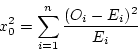
2. Define and develop a Poker test for four-digit random numbers. A sequence of 10,000 random numbers, each of four digits has been generated. The analysis of the numbers reveals that in 5120 numbers all four digits are different, 4230 contain exactly one pair of like digits, 560 contain two pairs, 75 have three digits of a kind and 15 contain all like digits. Use Poker test to determine whether these numbers are independent. (Critical value of chi-square test for α=0.05 and N=4 is 9.49)
The Poker Test is the test for independence based on the frequency with which certain digits are repeated with in a series of numbers. This test not only tests for the randomness of the sequence of numbers, but also the digits comprising of each of the numbers. The expected value of each of the combination of digits in a number is compared with the observed value by means of the chi-square test for independence. The acceptance is done if the observed value of chi-square sums for all the possible combinations of digits is less than the acceptable value for the given degree of freedom at the specified confidence interval.
Poker test for four digit numbers
In four digit number, there are five different possibilities
- All individual digits can be different
- There can be one pair of like digit
- There can be two pair of like digits
- There can be three digits of a kind
- There can be four digits of a kind
The probabilities associated with each of the possibilities is given by
P (four different digits) = 4C4 * (10/10) * (9/10) * (8/10) * (7/10) = 0.504
P (one pair) = 4C2 * (10/10) * (1/10) * (9/10) * (8/10) = 0.432
P (two pair) = (4C2/2)*(10/10) * (1/10) * (9/10) * (1/10) = 0.027
P (three digits of a kind) = 4C3 * (10/10) * (1/10) * (1/10) * (9/10) = 0.036
P (four digits of a kind) = 4C4 * (10/10) * (1/10) * (1/10) * (1/10) = 0.001
Now the calculation table for the Chi-square statistics is:
| Combination(i) | Observed Frequency(Oi) | Expected Frequency(Ei) | (Oi-Ei) | (Oi-Ei)2/Ei |
| Four different digits | 5120 | 0.504*10000 = 5040 | 80 | 1.269 |
| One pair | 4230 | 0.432*10000 = 4320 | -90 | 1.875 |
| Two pair | 560 | 0.027*10000 = 270 | 290 | 311.481 |
| Three digits of a kind | 75 | 0.036*10000 = 360 | 285 | 225.625 |
| Four digits of a kind | 15 | 0.001*10000 = 10 | 5 | 2.5 |
| 10000 | 10000 | Σ(Oi-Ei)2/Ei = 542.75 |
 = 542.75
and Given  α, N = 0.05, 4= 9.49
Here the calculated value of chi-square is 542.75 which is greater than the given tabulated value of chi- square so we reject the null hypothesis of independence between given numbers.
Group B
Short answer Questions:
Attempt
any eight questions. (5x8=40)
3. Define congestion in a queuing system. Describe different types of components and characteristics of a queueing system.
A congestion system is system in which there is a demand for resources for a system, and when the resources become unavailable, those requesting the resources wait for them to become available. The level of congestion in such systems is usually measured by the waiting line, or queue, of resource requests (waiting line or queuing models).
Characteristics/Elements of Queueing System
The key elements of queuing systems are customer and server. Customer refers to anything that arrives at a facility and requires service. E.g. people, machines, trucks, emails. Servers refers to any resource that provides the requested service. E.g. receptionist, tellor, CPU, washing machine etc.
1. Calling Population
The population of potential customers those require service from system is called calling population. It may be finite or infinite. System having large calling population is usually considered as infinite. For e.g. customers at banks, restaurant. And System having less and countable population is usually considered as finite. For e.g. a certain number of machines to be repaired by a service man.
In finite population model, arrival rate depends on the number of customers being served and waiting. But in infinite population model, arrival rate is not affected by the number of customer being served and waiting.
2. Arrival Process
The arrival process for infinite-population models is usually characterized in terms of interarrival times of successive customers. Arrivals may occur at scheduled times or at random times. When at random times, the inter arrival times are usually characterized by a probability distribution and most important model for random arrival is the poisson process. In schedule arrival interarrival time of customers are constant.
3. Service Process
Service process can be measured by the number of customers served per some unit of time or the time taken to complete the service. Once entities have entered to the system they must be served. The service can be provided in single or batch. if it is batch, as in the case of arrival the batch size can be fixed or random. Service time may be of constant duration or of random duration.
Markov Service process: A Markov service process is a special service process in which entities are processed one at a time in FCFS order and service times are independent and exponential. Aswith the case of Markov arrivals, a Markov service process is memoryless, which means that the expected time until an entity is finished remains constant regardless of how long it has been in service.
4. Queueing Discipline and Queueing Behaviour
Queue discipline refers to the rule that a server uses to choose the next customer from the queue when the server completes the service of the current customer. Common queue disciplines include first-in-first-out (FIFO); last-in-first-out (LIFO); service in random order (SIRO); shortest processing time first (SPT); and service according to priority (PR).
- First in first out :This principle states that customers are served one at a time and that the customer that has been waiting the longest is served first.
- Last in first out : This principle also serves customers one at a time, however the customer with the shortest waiting time will be served first.
- Service in random order: A customer is picked up randomly from the waiting queue for service.
- Shortest job first: The next job to be served is the one with the smallest size (shortest service time).
- Priority: Customers with high priority are served first.
Queue behavior refers to the actions of customers while in a queue waiting for service to begin. Different queue behaviours are:
- Balk/Balking: It means leaving the queue when the customer see the line is too long.
- Renege/Reneging: Leave after being in the line when they see that the line is moving too slowly.
- Jockey/Jockeying: Move from one to a shortest line.
5. Number of Servers:
Servers represent the entity that provides service to the customer. A system may consist of single server or multiple servers.
- A system with multiple servers is able to provide parallel services to the customers.
4. Define and describe different types of elements and components of a system.
A group of components which are interconnected and interact to fulfill certain objective is called a system. A system mainly consists of 4 elements: input, process, output and feedback.

Fig: Block diagram of system
Input: It involves capturing and assembling elements that enter the system to be processed. Inputs to the system are anything to be captured by the system from its environment. For example, raw materials.
Processing: It involves transformation processes that convert input to output. For example, a manufacturing process.
Output: It involves transferring elements that have been produced by a transformation process to their ultimate destinations. Outputs are the things produced by the system and sent into its environment. For example, finished products.
Feedback: It is the idea of monitoring the current system output and comparing it to the system goal. Any variation from the goal are then fed back in to the system and used to adjust it to ensure that it meets its goal. For example, data about sales performance is feedback to a sales manager.
A system boundary is a line that separates the system from the system environment. A change occuring outside the system may affect the performance of the system. Such changes are said to occur in the system environment. Therefore the system environment means anything outside the system boundary that may affect the system.
Components of the system
1. Entity: An entity is an object of interest for the purpose of the system study.
2. Attribute: The property or the characteristics of an entity is called attribute.
3. Activity: The time period of specified length is called activity. The activity changes the state of the system.
4. State: The state of a system is defined as the collection of variables necessary to describe the system at any time with respect to objectives of the study.
5. Event: The instantaneous occurance that may change the state of a system is called event. There are 2 types of event:
a) Endogenous Event: The event that occurs within the system and change the state of the system is called endogenous event.
b) Exogenous Event: The event that occurs outside the system but affects the state of the system is called exogenous event.
5. Describe the importance of differential/Partial differential equations in simulation.
The equation that consists of the higher order derivatives of the dependent variable is known as differential equations.
- The differential equation is said to be linear if any of the dependent variables and its derivatives have power of one and are multiplied by the constant.
E.g. M x’’ + D x’ + K x = K F(t)
where, M, D and K are constants; F(t) is the input to the system depending upon the independent variable t; x’’ and x’ are second and first order derivatives of dependent variable x.
- The differential equation is said to be non-linear if the dependent variable or any of its derivatives are raised to a power or are combined in other way like multiplication.
The differential equation is said to be partial if more than one independent variables occur in a differential equation.
-E.g. Equation of flow of heat in three dimensional body. It consists of four independent variables ( three dimensions and time ) and one dependent variable ( temperature ).
Necessity of differential equations:
1. Most physical and chemical process occurring in the nature involves rate of change, which requires differential equations to provide mathematical model.
2. It can be used to understand general effects of growth trends as differential equations can represent a growth rate.
6. What do you understand by interactive and feedback system in simulation? Explain.
Interactive System
Interactive systems are computer systems characterized by significant amounts of interaction between humans and the computer. Editors, CAD-CAM (Computer Aided Design-Computer Aided Manufacture) systems, and data entry systems are all computer systems involving a high degree of human-computer interaction. Games and simulations are interactive systems. Web browsers and Integrated Development Environments (IDEs) are also examples of very complex interactive systems.
Feedback System
The system takes feedback from the output i.e. input is coupled with output. A significant factor in the performance of many systems is that coupling occurs between the input and output of the system. The term feedback is used to describe the phenomenon.
One example of feedback system in which there is continuous control is the aircraft system. Here the input is a desired aircraft heading and the output is the actual heading. The gyroscope of the autopilot is able to detect the difference between the two headings. A feedback is established by using the difference to operate the control surface. Since change of heading will then affect the signal being used to control the heading.
The difference between the desired signal θt and actual heading θ0 is called the error signal, since it is a measure of the extent to which the system from the desired condition. It is denoted by є.


We also know that, in terms of angular acceleration

From equation (1), (2) & (3)

Dividing both sides by I, and making the following substitutions in equation (4)

 (where
  is damping factor)
This is a second order differential equation.
7. What do you understand by distributed lag model? explain with example.
Models that have the property of changing only at fixed interval of time is called distributed lag model. It is used to predict current values of a dependent variable based on both the current values of an explanatory variable (independent variable) and the lagged (past period) values of this explanatory variable.
This model consists of linear algebraic equations that represent continuous system but data are available at fixed points in time.
For example: Mathematical model of national economy
Let
C = consumption
I = investment
T = Taxes
G = government expenditures
Y = national income
Then
C=20+0.7(Y-T)
I=2+0.1Y
T=0.2Y
Y=C+I+G
All the equation are expressed in billions of rupees. This is static model and can be made dynamic by lagging all the variables as follows
C=20+0.7(Y-1-T-1)
I=2+0.1Y-1
T=0.2Y-1
Y=C-1+I-1+G-1
Any variable that can be expressed in the form of its current value and one or more previous value is called lagging variable. And hence this model is given the name distributed lag model. The variable in a previous interval is denoted by attaching –n suffix to the variable. Where –n indicate the nth interval.
8. Describe the process of calibration and validation in detail.
Validation is concerned with building the right model. It is utilized to determine that a model is an accurate representation of the real system. It is usually achieved through the calibration of the model.
Calibration means to validate the model with the real system, look out for the places for betterment of the models and revising the model to form next better model repeatedly until a satisfiable model is not achieved. The initial model is developed and is calibrated using Naylor-Finger calibration steps with the real system. It is then revised and a first revision model is generated. The first revision model is then calibrated with the real system. It is revised to form a second revision model. This process is continued until the model becomes acceptable.
Naylor and Finger formulated a three step approach:-
1. Build a model that has high face validity.
2. Validate model assumptions.
3. Compare the model input-output transformations to corresponding input-output transformations for the real system.
The following figure shows the relationship of the model calibration to the overall validation process.

The comparison of the model to reality is carried out by verity of test. Some test are subjective and other are objective.
- Subjective test usually involve people, who are knowledgeable about one or more aspects of the system, making judgments about the model and its output.
- Objective test always require data on the system's behavior plus the corresponding data produced by the model.
9. Draw and describe different types of GPSS blocks that are used to deal with queues?
GPSS (General Purpose Simulation System) is a highly structured and special purpose simulation language based on process interaction approach and oriented toward queuing systems.
- The system being simulated is described by the block diagram using various GPSS blocks.
- Each block represents events, delays or other actions that affect the transaction flow.
The two main blocks that are used with queues are QUEUE and DEPART.
QUEUE BLOCK:
This block will instruct GPSS to start gathering queuing statistics on the queue named in its attribute value. SYNTAX: QUEUE A
ATTRIBUTES: A = name of queue (for example: garage)

DEPART BLOCK:
This block instructs GPSS that a transaction is leaving the queue named in it‟s attribute value. This is necessary in order to compile the statistics on the queue.
SYNTAX: DEPART A
ATTRIBUTES: A = name of the queue (for example: checkout)

Some other blocks that are used with above blocks are:
GENERATE BLOCK:
This block will produce a flow of transactions with inter-arrival times determined by the attribute values. The distribution of inter-arrival times follows a uniform probability distribution.
SYNTAX: GENERATE A,B,C,D,E
ATTRIBUTES: A = average value of uniform distribution, B = half-width of uniform distribution, C = time delay before first transaction is generated, D = maximum number of transactions generated, E = priority allocated to transactions

ADVANCE BLOCK:
This block represents the servicing of a transaction. The servicing times follow a uniform probability distribution.
SYNTAX: ADVANCE A,B
ATTRIBUTES: A = average value of uniform distribution, B = half-width of uniform distribution

TERMINATE BLOCK:
This block destroys any transaction entering it and removes it from computer memory. Each time a transaction enters this block it decrements a counter by an amount equal to its attribute value. The counter is set by the user upon starting the simulation.
SYNTAX: TERMINATE A
ATTRIBUTES: A = decrements simulation counter by this amount

etc.
10. Differentiate between fixed time step and event to event model with the help of suitable examples.
Fixed time-step model
In this the timer simulated by the computer is updated at a fixed time interval. The system is checked to see if any event has taken place during that interval. All the events which take place during the time interval are considered to have occurred simultaneously at the end of the interval.
Event-to-event model
It is also known as the next-event model. In this the computer advances the time to the occurrence of the next event. So it shifts from one event to the next event and the system state does not change in between. A track of the current time is kept when something interesting happens to the system.
The flowcharts for both models is shown below.

11. Why do we need the analysis of simulation output? How do you use estimation method in output analysis? Explain.


 , Variance σ² and we have a sample of n size then the confidence interval is given by:
 is defined by
12. Write a computer program in C that will generate four digit random numbers using the multiplicative congruential method. Allow the user to input values of X0, a, c and m.
# include<stdio.h>
#include<conio.h>
#include<math.h>
int main()
{
int x[10], n, a, c, m, i, j;
float r[10];
printf("Enter the number of random number to generate:");
scanf("%d", &n);
printf("Enter the value of seed x0:);
scanf("%d", &x[0]);
printf("Enter the value of a:");
scanf("%d", &a);
printf("Enter the value of c:");
scanf("%d", &c);
printf("Enter the value of m:");
scanf("%d", &m);
i=0;
r[0] = float(x[0]/m);
if (c == 0 && m==10000){
do{
x[i+1] = (a*x[i])%m;
r[i+1] = float(x[i+1]/m);
i++;
}while(i<=n);
printf("The obtained random numbers are:");
for(j=0; j<n; j++)
{
printf("%f", &r[j];
}
else{
printf("For Multiplicative congruential method the value of c should be zero and to generate four digit random number the value of m should be 10000 !!");
}
return 0;
}
13. Define and describe Markov Chain with example.
If the future states of a process are independent of the past and depend only on the present , the process is called a Markov process. A discrete state Markov process is called a Markov chain. A Markov Chain is a random process with the property that the next state depends only on the current state.
Markov chains are used to analyze trends and predict the future. (Weather, stock market, genetics, product success, etc.
Formally,
A Markov chain is a sequence of random variables X1, X2, X3, ... with the Markov property, namely that, given the present state, the future and past states are independent.

The conditional probability above gives us the probability that a process in state in at time n moves to in+1 at time n + 1. We call this the transition probability for the Markov chain. If the transition probability does not depend on the time n, we have a stationary Markov chain, with transition probabilities

Now we can write down the whole Markov chain as a matrix P:

Example:
Weather Problem:
- raining today ⇒ 40 % rain tomorrow
⇒ 60 % no rain tomorrow
- not raining today ⇒ 20 % rain tomorrow
⇒ 80 % no rain tomorrow
What will be probability if todays is not raining then not rain the day after tomorrow?
Markov chain diagram:

Transition matrix:


Thus, the probability of not rainy the day after tomorrow is 0.76.