Simulation and Modelling 2074
Group A
Long Answer Questions:
Attempt
any two questions.
(2x10=20)
1. Differentiate between static and dynamic physical models in simulation. Describe dynamic physical model in detail with the help of suitable example.
Static Physical Model
- Static physical model is the physical model which describes relationships that do not change with respect to time.
- Such models only depict the object’s characteristics at any instance of time, considering that the object’s property will not change over time.
- Eg : An architectural model of a house, scale model of a ship and so on.
Dynamic Physical Model
- Dynamic physical model is the physical model which describes the time varying relationships of the object properties.
- Such models describes the characteristics of the object that changes over time.
- It rely upon the analogy between the system being studied and some other system of a different nature, but have similarity on forces that directs the behavior of the both systems.
- Eg: A model of wind tunnel, a model of automobile suspension and so on.
To illustrate this type of physical model, consider the two systems shown in following figures i.e. Figure 1 and Figure 2.

Fig1: Mechanical System

Fig2: Electrical system
The Figure 1. represents a mass that is subject to an applied force F(t) varying with time, a spring whose force is proportional to its extension or contraction, and a shock absorber that exerts a damping force proportional to the velocity of the mass.It can be shown that the motion of the system is described by the following differential equation.

Where,
x is the distance moved, M is the mass, K is the stiffness of the spring & D is the damping factor of the shock absorber.
Figure 2. represents an electrical circuit with an inductance L, a resistance R, and a capacitance C, connected in series with a voltage source that varies in time according to the function E(t). If q is the charge on the capacitance, it can be shown that the behavior of the circuit is governed by the following differential equation:

Inspection of these two equations shows that they have exactly the same form and that the following equivalences occur between the quantities in the two systems:
a) Displacement x = Charge q
b) Velocity x’ = Current I, q’
c) Force F = Voltage E
d) Mass M = Inductance L
e) Damping Factor D = Resistance R
f) Spring stiffness K = Inverse of Capacitance 1/C
g) Acceleration x’’ = Rate of change of current q’’
The mechanical system and the electrical system are analogs of each other, and the performance of either can be studied with the other.
2. Use multiplicative congruential method to generate a sequence of three digits random numbers between (0, 1) with X0=27, a=3 and m=1000. Use any one of the uniformity test to find out whether the generated numbers are uniformly distributed or not? (Critical value for α=0.05 and N=5 is 0.565).
Given,
X0 = 27,
α = 3,
m=1000
We have,
For multiplicative congruential method:
Xi+1 = (α Xi ) mod m
& Ri =Xi/m,
The sequence of random numbers are calculated as follows:
X0 = 27
R0 = 27/1000 = 0.027
X1 = (α X0) mod m = (3*27) mod 1000 = 81 mod 1000 = 81
R1 = 81/1000 = 0.081
X2 = (α X1) mod m = (3*81) mod 1000 = 243 mod 1000 = 243
R2 = 243/1000 = 0.243
X3 = (α X2) mod m = (3*243) mod 1000 = 729 mod 1000 = 729
R3 = 729/1000 = 0.729
X4= (α X3 ) mod m = (3*729) mod 1000 = 2187 mod 1000 = 187
R4 = 187/1000 = 0.187
Arranging the above random numbers number in ascending order:
0.027, 0.081, 0.187, 0.243,, 0.729
Here, N = 5
Calculation table for Kolmogorov-Smirnov test :
| i |  |  |  |  |
| 1 | 0.027 | 0.2 | 0.173 | 0.027 |
| 2 | 0.081 | 0.4 | 0.319 | - |
| 3 | 0.187 | 0.6 | 0.413 | - |
| 4 | 0.243 | 0.8 | 0.557 | - |
| 5 | 0.729 | 1 | 0.271 | - |
Now, calculating
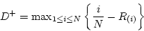 = 0.557
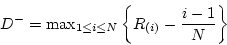 = 0.027
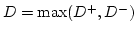 = 0.557
Given, Critical value  = 0.565
Since the computed value, D = 0.557, is less than the tabulated critical value, = 0.565, the hypothesis of no difference between the distribution of the generated numbers and the uniform distribution is not rejected.
3. Why is GPSS called transaction flow oriented language? A machine tool in a manufacturing shop is turning out parts at the rate of every 5 minutes. When they are finished, the parts are sent to an inspector, who takes 4±3 minutes to examine each one and rejects 20% of the parts. Draw and explain a block diagram for it and write a GPSS program to simulate using the concept of FACILITY.
GPSS (General Purpose Simulation System) is a highly structured and special purpose simulation language based on process interaction approach and oriented toward queuing systems. The system being simulated is described by the block diagram using various GPSS blocks. Each block represents events, delays or other actions that affect the transaction flow. Therefore GPPS is called transaction flow oriented language.
The block diagram for given problem using GPSS is given below:

A GENERATE block is used to represent the output of the machine by creating one transaction every five units of time. A QUEUE block places the transaction in the queue and SEIZE block allows a transaction to engage a facility if it is available. If more than one inspector is available, the transaction leaves the queue which is denoted by DEPART block and enters into ADVANCE block. An ADVANCE block with a mean of 4 and modifier of 3 is used to represent inspection. The time spent on inspection will therefore be any one of the values 1, 2, 3, 4, 5, 6 or 7, with equal probability given to each value. Upon completion of the inspection, RELEASE block allows a transaction to disengage the facility and transaction go to a TRANSFER block with a selection factor of 0.2, so that 80 % of the parts go to the next location called ACC, to represent accepted parts and 20 % go to another location called REJ to represent rejects. Both locations reached from the TRANSFER block are TERMINATE blocks.
Now,
Code for simulating the given problem using GPSS:
GENERATE 5, 0
QUEUE 1
SEIZE 1
DEPART 1
ADVANCE 4, 3
RELEASE 1
TRANSFER 0.2 ACC REJ
ACC TERMINATE 1
REJ TERMINATE 1
Group B
Short answer Questions:
Attempt
any eight questions. (5x8=40)
4. Differentiate between numerical and analytical methods in system simulation.
| Analytical Method | Numerical Method |
| Analytical method is one which is solved by using the deductive reasoning of mathematical theory. | Numerical method is the one which is solved by applying computational procedures. |
| Analytical method provide a direct solution and will result in exact solution if one exists. | Numerical method often require many iterations to get true solution. |
| Analytical method is exact and gives exact solution. E.g. value of 1/2 | Numerical method gives the approximate value or solution. E.g. PI=22/7 is approximate value. |
| Analytical methods are time consuming and sometimes impossible. | Mathematical methods are less time consuming and possible for most cases. |
| This model is best for designing calculations, suit for checking calculation with certain limitation. | This model is best for checking calculations, practically effective for designing calculation. |
| This model is not versatile & flexible . | This model is versatile and flexible. |
| Need much work to be developed, but only simple software for application. | Need expensive and complex software and hardware. |
5. Describe different phases of simulation study with the help of flow chart.
Phases of Simulation Study

I Phase:
- Consists of steps 1 and 2
- It is period of discovery/orientation
- The analyst may have to restart the process if it is not fine-tuned
- Recalibrations and clarifications may occur in this phase or another phase.
II Phase:
- Consists of steps 3,4,5,6 and 7
- A continuing interplay is required among the steps
- Exclusion of model user results in implications during implementation
III Phase:
- Consists of steps 8,9 and 10
- Conceives a thorough plan for experimenting
- Discrete-event stochastic is a statistical experiment
- The output variables are estimates that contain random error and therefore proper statistical analysis is required.
IV Phase:
- Consists of steps 11 and 12
- Successful implementation depends on the involvement of user and every steps successful completion.
6. Define random numbers and describe why the random numbers generated by computer called pseudo random numbers?
- Random numbers are samples drawn from a uniformly distributed random variable between some satisfied intervals, they have equal probability of occurrence.
- A number chosen from some specified distribution randomly such that selection of large set of these numbers reproduces the underlying distribution is called random number.
In computer random numbers are derived from a known starting point and is typically repeated over and over using some known methods (algorithms) to produce a sequence of numbers. The sequence of numbers are not completely random as the set of random numbers can be replicated because of use of some known method. So, the random numbers generated by computer called pseudo random numbers.
Every new number is generated from the previous ones by an algorithm. This means that the new value is fully determined by the previous ones. But, depending on the algorithm, they often have properties making them very suitable for simulations.
When generating pseudo-random numbers, certain problems or errors can occur. Some examples include the following:
1. The generated numbers might not be uniformly distributed.
2. The generated numbers might be discrete valued instead of continuous valued.
3. The mean of the generated numbers might be too high or too low.
4. The variance of the generated numbers might be too high or too low.
5. There might be presence of correlation between the generated numbers.
7. Define confidence interval and I.I.D in output analysis. How do you use simulation run statistics in simulation output analysis? Explain.
Example:
Consider a system with Kendall’s notation M/M/1/FIFO (i.e. a single server system in which the inter-arrival time is distributed exponentially ;and service time has an exponential and queue discipline is FIFO) and the objective is to measure the mean waiting time.
In simulation run approach, the mean waiting time is estimated by accumulating the waiting time of n successive entities and then it is divided by n. This measures the sample mean such that:

Whenever a waiting line forms, the waiting time of each entity on the line clearly depends upon the waiting time of its predecessors. Such series of data in which one value affect other values is said to be autocorrelated. The sample mean of autocorrelated data can be shown to approximate a normal distribution as the sample size increases.
A simulation run is started with the system in some initial state, frequently the idle state, in which no service is being given and no entities are waiting. The early arrivals then have a more than normal probability of obtaining service quickly, so a sample mean that includes the early arrivals will be biased.
8. Describe the process of model building, verification and validation in detail.
Verification is concerned with building the model right. It is utilized in comparison of the conceptual model to the computer representation that implements that conception.
Validation is concerned with building the right model. It is utilized to determine that a model is an accurate representation of the real system. It is usually achieved through the calibration of the model.

Fig: Model building, verification and validation
1.The first step in model building consists of observing the real system and the interactions among its various components and collecting data on its behavior.
2.The second step in model building is the construction of a conceptual model – a collection of assumptions on the components and the structure of the system, plus hypotheses on the values of model input parameters, illustrated by the above figure.
3.The third step is the translation of the operational model into a computer recognizable form- the computerized model.
Model building, verification and validation is not a linear process. Will return to each many step while building, verification and validation of model.
9. Define traffic intensity and server utilization. Write down the Kendall’s notation for queuing system with example.
Traffic Intensity
The ratio of the mean service time to the mean inter arrival time is called traffic intensity. I.e. u= λ"Ts or u=Ts/Ta
Server Utilization
Server utilization is the percentage of the time that all servers are busy. Server utilization factor (ρ ) is the ratio of average arrival rate (λ) to the average service rate (μ).
ρ = λ/μ in the case of a single server model
ρ = λ/μn in the case of a “n” server model
Kendall's notation
Kendall’s notation is used for parallel server systems. The basic format of this notation is of form: A / B / c / N / K, where, A, B, c, N, K respectively indicate arrival pattern, service pattern, number of servers, system capacity, and Calling population.
The symbols used for the probability distribution for inter arrival time, and service time are, D for deterministic, M for exponential (or Markov) and Ek for Erlang.
E.g.
a) M/D/2/5/∞ stands for a queuing system having exponential arrival times, deterministic service time, 2 servers, capacity of 5 customers, and infinite population.
b) M/D/2 means exponential arrival time, deterministic service time, 2 servers, infinite service capacity, and infinite population.
10. What do you understand by queueing and queueing discipline? An office works for 5 days, 8 hours per day, and receives 1200 telephone call in the week. Calculate the mean arrival rate and mean inter-arrival time of the calls.
The line where the entities or customer wait is generally known as queue. The combination of all entities in system being served and being waiting for service will be called as queueing system.
Queue discipline refers to the rule that a server uses to choose the next customer from the queue when the server completes the service of the current customer. Common queue disciplines include first-in-first-out (FIFO); last-in-first-out (LIFO); service in random order (SIRO); shortest processing time first (SPT); and service according to priority (PR).
- First in first out :This principle states that customers are served one at a time and that the customer that has been waiting the longest is served first.
- Last in first out : This principle also serves customers one at a time, however the customer with the shortest waiting time will be served first.
- Service in random order: A customer is picked up randomly from the waiting queue for service.
- Shortest job first: The next job to be served is the one with the smallest size (shortest service time).
- Priority: Customers with high priority are served first.
Now,
Mean arrival rate = λ
Mean inter-arrival time = Ta
Total working hours = 5 * 8 = 40 hrs per week
Total calls in the week = 1200
Ta = (40*60*60 sec)/1200 = 144,000 sec/1200 = 120 sec = 2 min
λ = 1/Ta = 1/2 = 0.5 call per min
11. What is absolute clock and relative clock time in GPSS? How do you update the clock time in simulation? Explain.
Absolute clock measures the simulated time that has elapsed since the simulation began.
Relative clock tells how much simulated time has elapsed since a RESET statement was most recently executed. The relative clock has no special meaning unless one or more RESET run-control statements are used in the model file.
When there are no RESET statements in a model file, the RELATIVE and ABSOLUTE CLOCKS have identical values.
Clock time is updated based on the following two models:
1. Fixed time-step model
In this the timer simulated by the computer is updated at a fixed time interval. The system is checked to see if any event has taken place during that interval. All the events which take place during the time interval are considered to have occurred simultaneously at the end of the interval.
2. Event-to-event model
It is also known as the next-event model. In this the computer advances the time to the occurrence of the next event. So it shifts from one event to the next event and the system state does not change in between. A track of the current time is kept when something interesting happens to the system.
The flowcharts for both models is shown below.

12. Write a computer program that will generate three digit random numbers using the linear congruential method. Allow the user to input values of X0, a, c and m.
# include<stdio.h>
#include<conio.h>
#include<math.h>
int main()
{
int x[10],n, a, c, m, i, j;
float r[10];
printf("Enter the number of random number to generate:");
scanf("%d", &n);
printf("Enter the value of seed x0:);
scanf("%d", &x[0]);
printf("Enter the value of a:");
scanf("%d", &a);
printf("Enter the value of c:");
scanf("%d", &c);
printf("Enter the value of m:");
scanf("%d", &m);
i=0;
r[0] = float(x[0]/m);
if (m ==1000)
{
do{
x[i+1] = (a*x[i]+c)%m;
r[i+1] = float(x[i+1]/m);
i++;
}while(i<=n);
printf("The obtained random numbers are:");
for(j=0; j<n; j++)
{
printf("%f", &r[j];
}
else{
printf("To generate three digit random number the value of m should be 1000 !!");
}
return 0;
}
13. Define CSMP. Describe different types of statements in CSMP with example.
CSMP or Continuous System Modelling Program is an early scientific computer software designed for modelling and solving differential equations numerically. This enables real-world systems to be simulated and tested with a computer.
Types of statements in CSMP
1. Structural statements which defines the model. They consist of FORTARN like statement and functional block designed for operations that frequently occur in a model definition. Structural statement can make use of the operation of addition, subtraction, multiplication, division and exponentiation, using the same notation and rule as are used in FORTRAN. If the model include the equation  .Then the following statement would be used
X=6.0*Y/W+(Z-2)**2.0
2. Data statements which assign numerical value to parameters, constant and initial conditions. For example one data statement called INCON can be used to set the initial value of integration function block.
3. Control statements which specify options in the assembly and execution of program and choice of inputs. For e.g. If printed output is required, control statements with PRINT and PRDEL are used followed by the names of variables to form the outputs.