Simulation and Modelling Model Question
Section A
Attempt any two questions. (2 × 10 = 20)
1. What are the characteristics of Queuing System? What are the various performance
measures in single server (M/M/1) queuing system simulation? (5 +5)
Characteristics of Queueing System
1. Calling Population
The population of potential customers those require service from system is called calling population. It may be finite or infinite. System having large calling population is usually considered as infinite. For e.g. customers at banks, restaurant. And System having less and countable population is usually considered as finite. For e.g. a certain number of machines to be repaired by a service man.
In finite population model, arrival rate depends on the number of customers being served and waiting. But in infinite population model, arrival rate is not affected by the number of customer being served and waiting.
2. Arrival Process
The arrival process for infinite-population models is usually characterized in terms of interarrival times of successive customers. Arrivals may occur at scheduled times or at random times. When at random times, the inter arrival times are usually characterized by a probability distribution and most important model for random arrival is the poisson process. In schedule arrival interarrival time of customers are constant.
3. Service Process
Service process can be measured by the number of customers served per some unit of time or the time taken to complete the service. Once entities have entered to the system they must be served. The service can be provided in single or batch. if it is batch, as in the case of arrival the batch size can be fixed or random. Service time may be of constant duration or of random duration.
Markov Service process: A Markov service process is a special service process in which entities are processed one at a time in FCFS order and service times are independent and exponential. Aswith the case of Markov arrivals, a Markov service process is memoryless, which means that the expected time until an entity is finished remains constant regardless of how long it has been in service.
4. Queueing Discipline and Queueing Behaviour
Queue discipline refers to the rule that a server uses to choose the next customer from the queue when the server completes the service of the current customer. Common queue disciplines include first-in-first-out (FIFO); last-in-first-out (LIFO); service in random order (SIRO); shortest processing time first (SPT); and service according to priority (PR).
- First in first out :This principle states that customers are served one at a time and that the customer that has been waiting the longest is served first.
- Last in first out : This principle also serves customers one at a time, however the customer with the shortest waiting time will be served first.
- Service in random order: A customer is picked up randomly from the waiting queue for service.
- Shortest job first: The next job to be served is the one with the smallest size (shortest service time).
- Priority: Customers with high priority are served first.
Queue behavior refers to the actions of customers while in a queue waiting for service to begin. Different queue behaviours are:
- Balk/Balking: It means leaving the queue when the customer see the line is too long.
- Renege/Reneging: Leave after being in the line when they see that the line is moving too slowly.
- Jockey/Jockeying: Move from one to a shortest line.
5. Number of Servers:
Servers represent the entity that provides service to the customer. A system may consist of single server or multiple servers.
- A system with multiple servers is able to provide parallel services to the customers.
The various performance measures in single server (M/M/1) queuing system simulation is discussed below:
1. If Ta and Ts be the inter arrival time and the mean service time then
- Arrival rate λ=1/Ta
- Service rate μ=1/Ts
2. The ratio of the mean service time to the mean inter arrival time is called traffic intensity. i.e. u=Ts/Ta
3. Server utilization: It consists of only the arrival that gets served. It is denoted by and defined as
ρ= λTs= λ/ μ (server utilization for single server).
4. Probability of finding service counter free is (1 – ρ) i.e there are zero customers in the service facility.
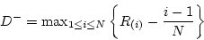
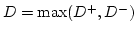
2. Differentiate between true and pseudo random numbers. What are the basic properties of random numbers? The sequence of numbers 0.37, 0.29, 0.19, 0.88 0.44, 0.63, 0.77, 0.70 0.21, and 0.58 has been generated. Use K-S test to determine if the numbers are uniformly distributed (Dα = 0.41 for α = 0.05 (2 + 2 + 6)
Difference between true and pseudo random numbers
- Pseudo random numbers are the random numbers that are generated by using some known methods (algorithms) so as to produce a sequence of numbers in [0,1] that can simulates the ideal properties of random numbers. They are not completely random as the set of random numbers can be replicated because of use of some known method.
- True random numbers are gained from physical processes like radioactive decay or also rolling a dice and introduce it into a computer.
- Pseudo random numbers have fast response in generating numbers while true random have slow response.
- In pseudo random number, sequence of numbers can be reproduced where as In true random number, sequence of numbers can't be reproduced.
- In pseudo random number, sequence of number is repeated where as In true random number, sequence of numbers will or will not be repeated.
Properties of Random Numbers
1. Uniformity:
- The random numbers generated should be uniform. That means a sequence of random numbers should be equally probable every where.
- If we divide all the set of random numbers into several numbers of class interval then number of samples in each class should be same.
- If ‘N’ number of random numbers are divided into ‘K’ class interval, then expected number of samples in each class should be equal to ei = N / K.
2. Independent:
- Each random number should be independent samples drawn from a continuous uniform distribution between 0 and 1.
- The probability density function is given by:
f(x) = 1, 0 <= x <= 1
= 0, otherwise
3. Maximum Density:
- The large samples of random number should be generated in a given range.
4. Maximum Cycle:
- It states that the repetition of numbers should be allowed only after a large interval of time.
Now,
Given sequence of number,
0.37, 0.29, 0.19, 0.88 0.44, 0.63, 0.77, 0.70 0.21, and 0.58
Arranging the given number in ascending order:
0.19, 0.21, 0.29, 0.37, 0.44, 0.58, 0.63, 0.7, 0.77, 0.88
Here, N = 10
Calculation table for Kolmogorov-Smirnov test :
| i |  |  |  |  |
| 1 | 0.19 | 0.1 | - | 0.19 |
| 2 | 0.21 | 0.2 | - | 0.11 |
| 3 | 0.29 | 0.3 | 0.01 | 0.09 |
| 4 | 0.37 | 0.4 | 0.03 | 0.07 |
| 5 | 0.44 | 0.5 | 0.06 | 0.04 |
| 6 | 0.58 | 0.6 | 0.02 | 0.08 |
| 7 | 0.63 | 0.7 | 0.07 | 0.03 |
| 8 | 0.7 | 0.8 | 0.1 | - |
| 9 | 0.77 | 0.9 | 0.13 | - |
| 10 | 0.88 | 1.0 | 0.12 | - |
Now, calculating
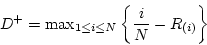 = 0.13
 = 0.19
 = 0.19
Given, Critical value  = 0.41
Since the computed value, D = 0.19, is less than the tabulated critical value, = 0.41, the hypothesis of no difference between the distribution of the generated numbers and the uniform distribution is not rejected.
3. Explain the analogy between Mechanical system and electrical system using Dynamic
Physical Model. Explain Dynamic mathematical model and static mathematical model.
Analogy between Mechanical system and electrical system
Consider the two systems shown in following figures i.e. Figure 1 and Figure 2.

Fig1: Mechanical System

Fig2: Electrical system
The Figure 1. represents a mass that is subject to an applied force F(t) varying with time, a spring whose force is proportional to its extension or contraction, and a shock absorber that exerts a damping force proportional to the velocity of the mass.It can be shown that the motion of the system is described by the following differential equation.

Where,
x is the distance moved, M is the mass, K is the stiffness of the spring & D is the damping factor of the shock absorber.
Figure 2. represents an electrical circuit with an inductance L, a resistance R, and a capacitance C, connected in series with a voltage source that varies in time according to the function E(t). If q is the charge on the capacitance, it can be shown that the behavior of the circuit is governed by the following differential equation:

Inspection of these two equations shows that they have exactly the same form and that the following equivalences occur between the quantities in the two systems:
a) Displacement x = Charge q
b) Velocity x’ = Current I, q’
c) Force F = Voltage E
d) Mass M = Inductance L
e) Damping Factor D = Resistance R
f) Spring stiffness K = Inverse of Capacitance 1/C
g) Acceleration x’’ = Rate of change of current q’’
The mechanical system and the electrical system are analogs of each other, and the performance of either can be studied with the other.
Static Mathematical Model
- Static mathematical model is the mathematical model that represents the logical view of the system in equilibrium state.
- Such models are time-invariant.
- It is generally represented by the basic algebraic equations.
- E.g. An equation relating the length and weight on each side of a playground variation, supply and demand relationship model of a market and so on.
Dynamic Mathematical Model:
- Dynamic mathematical model is the mathematical model that accounts for the time dependent changes in the logical state of the system.
- Such models are time-variant.
- It is generally represented by differential equations or difference equations.
- E.g. The equation of motion of planets around the sun in the solar system.
Section B
Attempt ANY EIGHT questions. (8 × 5 = 40)
4. Explain about system, its environment and its components.
A group of components which are interconnected and interact to fulfill certain objective is called a system. A system mainly consists of input, process, output and feedback.

Fig: Block diagram of system
A system boundary is a line that separates the system from the system environment. A change occuring outside the system may affect the performance of the system. Such changes are said to occur in the system environment. Therefore the system environment means anything outside the system boundary that may affect the system.
Components of the system
1. Entity: An entity is an object of interest for the purpose of the system study.
2. Attribute: The property or the characteristics of an entity is called attribute.
3. Activity: The time period of specified length is called activity. The activity changes the state of the system.
4. State: The state of a system is defined as the collection of variables necessary to describe the system at any time with respect to objectives of the study.
5. Event: The instantaneous occurance that may change the state of a system is called event. There are 2 types of event:
a) Endogenous Event: The event that occurs within the system and change the state of the system is called endogenous event.
b) Exogenous Event: The event that occurs outside the system but affects the state of the system is called exogenous event.
5. What is analog computer? Design a basic analog computer that represents a simple
dynamic system.
Analog computers are those computers that are unified with devices like adder and integral so as to simulate the continuous mathematical model of the system, which generates continuous outputs.
Analog method of system simulation is for use of analog computer and other analog devices in the simulation of continuous system. The analog computation is sometimes called differential analyser. Electronics analog computers for simulation are based on the use of high gain dc amplifiers called operational amplifier (op amps). In such analog computer, voltages are equated to mathematical variables and the op amps can add and integrate the voltages. The proper configurations can handle addition of several input voltages each representing the input variables. The analog computer provides limited accuracy because op amps have many assumptions which can never be true in reality.
Now,
Designing analog computer for Automobile Suspension system:
The general method by which analog computers are applied can be demonstrated using second order differential equation.
M x" + D x' + K x = K F(t)
Solving the equation for the highest order derivate gives,
M x" = K F(t) – D x' - K x

Fig: Automobile suspension problem
Suppose a variable representing the input F(t) is supplied, assume there exist variables representing -x and -x'. These three variables can be scaled and added to produce Mx". Integrating it with a scale factor 1/M produces X'. Changing sign produces -x', further integrating produces -x, a further sign inverter is included to produce +x as output.
6. What is non-stationary Poisson process? How can we convert it into a stationary Poisson
process?
The non-stationary Poisson process is a Poisson process for which the arrival rate varies with time. More specifically, it can be defined as follows:
The counting process N(t) is a non-stationary Poisson process if:
a) The process has independent increments.
b) 
Where, λ(t) = the arrival rate at time t
dt = differential sized interval
The definition is identical to the stationary Poisson process, with the exception that the arrival rate, λ(t), is now a function of time.
A counting process N(t) is a stationary Poisson process with rate λ if
a) The process has independent increments.
b) The process has stationary increments. and
c) 
A non-stationary Poisson process can be transformed into a stationary Poisson process with arrival rate 1.
7. Explain Monte Carlo simulation method with an example.
Following are the three important characteristics of Monte-Carlo method:
- Its output must generate random samples.
- Its input distribution must be known.
- Its result must be known while performing an experiment.
Flowchart for Monte Carlo simulation:
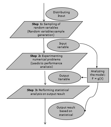
Fig: Flowchart of Monte Carlo simulation
Example:
Determining the value of PI using Monte Carlo method:


We use random number generation method to determine the sample points that lie inside or outside the curve. Let (x0, y0) be an initial guess for the sample point than from a linear congruential method of random number generation:
Xi+1 = (axi+c) mod m
Yi+1 = (ayi+c) mod m
Where a & c are constants, m is the upper limit of generated random number. If y<=yi then increment n.
8. Explain the three step approach of validation of models in simulation
Naylor and Finger proposed three step approach for validation process. These steps are as follows:
1. Face Validity
2. Validate Model Assumptions
3. Input - Output Transformation
1. Face validity
- A model should appear reasonable on its face to model users and to those who knows about the real system that is being simulated.
- A model should be designed with high degree of realism regarding system structure and behaviour through reliable data.
- The potential users should also be involved in the validation process to aid in identification of model deficiencies and optimizing those deficiencies to produce better model. This process is termed as structural walkthrough.
- Sensitivity analysis is also used for face validity of the model. It analyses the effect on output when there is change in input parameters. Sensitivity analysis is done through appropriate statistical techniques.
2. Model Assumptions
Model assumptions fall into two categories: structural assumptions and data assumptions.
- Structural assumptions involve questions of how the system operates and usually involve simplification and abstractions of reality.
- Data assumptions should be based on the collection of reliable data and correct statistical analysis of the data. It deals with such questions as what kind of input data model is? What are the parameter values to the input data model?
3. Input-Output Transformations:
- It involves validating whether the model can predict the future behaviour of the real system when the model input data match the real inputs and when a policy implemented in the model is implemented at some point in the system.
- In this validation phase, the model accepts values of the input parameters and transforms them into output measures of performance.
- The modeler uses the historical data reserved for validation purposes only.
- For the complete input-output validation, at least one set of input conditions should be collected from the system data so as to compare to model prediction.
9. Use Multiplicative congruential method to generate a sequence of 10 three-digit random
integers and corresponding random variables. Let X0 = 5, a = 3 and c=2.
Given,
X0 = 5,
α = 3
c = 2,
For three-digit random integers
m=1000
We have,
For multiplicative congruential method ( c =0) so
Xi+1 = (α Xi ) mod m
The sequence of random integers are calculated as follows:
X0 = 5
R0 = 5/1000 = 0.005
X1 = (α X0) mod m = (3*5) mod 1000 = 15 mod 1000 = 15
R1 = 15/1000 = 0.015
X2 = (α X1) mod m = (3*15) mod 1000 = 45 mod 1000 = 45
R2 = 45/1000 = 0.045
X3 = (α X2) mod m = (3*45) mod 1000 = 135 mod 1000 = 135
R3 = 135/1000 = 0.135
X4= (α X3 ) mod m = (3*135) mod 1000 = 405 mod 1000 = 405
R4 = 405/1000 = 0.405
X5= (α X4 ) mod m = (3*405) mod 1000 = 1215 mod 1000 = 215
R5= 215/1000 = 0.215
X6= (α X5) mod m = (3*215) mod 1000 = 645 mod 1000 = 645
R6 = 645/1000 = 0.645
X7= (α X6) mod m = (3*645) mod 1000 = 1935 mod 1000 = 935
R7 = 935/1000 = 0.935
X8= (α X7) mod m = (3*935) mod 1000 = 2805 mod 1000 = 805
R8 = 805/1000 = 0.805
X9= (α X8) mod m = (3*805) mod 1000 = 2415 mod 1000 = 415
R9 = 415/1000 = 0.415
X10 = (α X9) mod m = (3*415) mod 1000 = 1245 mod 1000 = 245
R10 = 245/1000 = 0.245
10. Why Confidence interval is needed in the analysis of simulation output. How can we can
we establish a confidence interval?
The confidence interval is the range of possible values for the parameter based on a set of data (e.g. the simulation results.). Confidence interval is needed because:
- A confidence interval displays the probability that a parameter will fall between a pair of values around the mean.
- Confidence intervals measure the degree of uncertainty or certainty in a sampling method.
Confidence intervals are based on the premise that the data being produced by the simulation is represented well by a probability model. Suppose the model is the normally distributed with mean  , Variance
  and we have a sample of n size then the confidence interval is given by:

In practice, the population variance is usually not known; in this case variance is replaced by the estimate calculated by the formula

This has a student t-distribution, with n – 1 degree of freedom. In terms of estimated variance S2, the confidence interval for  is defined by

Here, the quantity  is found on the student t-distribution table.
Example:
Suppose, the daily production time of a product in a factory for 120 days is 5.8 hours and sample standard deviation (S) is 1.6.
Now, confidence interval for 95% confidence level is calculated as;

[t119, 0.025 = 1.98]
Hence, the estimates between  can be accepted for 95% confidence interval.
11. Create a GPSS model and program to simulate a barber shop for a day (9am to 4pm),
where a costumer enters the Shop every 10 ± 2 minutes and a barber takes 13 ± 2 for a
haircut.
GPSS model to simulate a barber shop

Program
GENERATE 10,2
QUEUE SEAT
SEIZE BARBER
DEPART SEAT
ADVANCE 15,3
RELEASE BARBER
TERMINATE
TIMER GENERATE 420
TERMINATE 1
12. Write short notes on: (2 × 2.5 = 5)
a. Differential equation
b. Markov Chain
a. Differential equation
The equation that consists of the higher order derivatives of the dependent variable is known as differential equations.
- The differential equation is said to be linear if any of the dependent variables and its derivatives have power of one and are multiplied by the constant.
E.g. M x’’ + D x’ + K x = K F(t)
where, M, D and K are constants; F(t) is the input to the system depending upon the independent variable t; x’’ and x’ are second and first order derivatives of dependent variable x.
- The differential equation is said to be non-linear if the dependent variable or any of its derivatives are raised to a power or are combined in other way like multiplication.
The differential equation is said to be partial if more than one independent variables occur in a differential equation.
-E.g. Equation of flow of heat in three dimensional body. It consists of four independent variables ( three dimensions and time ) and one dependent variable ( temperature ).
b. Markov Chain
If the future states of a process are independent of the past and depend only on the present , the process is called a Markov process. A discrete state Markov process is called a Markov chain. A Markov Chain is a random process with the property that the next state depends only on the current state.
Markov chains are used to analyze trends and predict the future. (Weather, stock market, genetics, product success, etc).